
In this tutorial, we will be using Jupyter Notebook, Pandas and Plotly to explore and visualize the official IMDB dataset. You will learn how to apply common data science techniques such as data cleaning, filtering and visualization.
Introduction
Jupyter notebook and Pandas are great tools for data analysis. For a quick introduction to Pandas check out their 10 minutes to pandas guide. Another great tutorial is the Pandas Cookbook by Julia Evans. It starts from the very basics and digs into some great real-world data examples.
Once you're familiar with the fundamentals, you might wonder what other real-world datasets you could start exploring to hone your new skills. In this case you should take a look at the official IMDB datasets! They are available for personal and non-commercial use and contain millions of rows of real data from their website.
Apart from being interesting to explore, another great thing about these datasets is that there are some flaws in the data format. This means that before you can really get started, you will have to do some data cleaning. As most of the datasets in the real world are not perfect, this is a very useful skill to learn and to practice! We will spend a bit of time to go through this process step by step.
In this tutorial, I will be using the command line to set up the environment. If that's something you are not familiar with, check out the Djangogirls Command Line Introduction.
As always, you can find the corresponding Jupyter notebook file on Github.
WARNING: The IMDb dataset is quite large, so make sure you have enough free memory on your machine. On my setup running the notebook takes about 3-4 GB of RAM.
Setup
Create a new a project folder and virtual environment. Activate the virtual environment and install Jupyter notebook and Pandas using pip.
$ mkdir imdbexplore && cd imdbexplore
$ python -m venv .venv
$ source .venv/bin/activate  # macOS
$ .venv\Scripts\Activate.ps1  # Windows
$ (.venv) pip install notebook pandas
Download the IMDB datasets from their website. You can either do it from your browser or directly from the command line, as shown below.
There are a couple of different datasets available. We will be using the title.basics, which contains some basic information about movies like type, title, year, runtime, genre etc. The title.ratings dataset contains average ratings and rating count for movies.
# Windows
wget https://datasets.imdbws.com/title.basics.tsv.gz
wget https://datasets.imdbws.com/title.ratings.tsv.gz
# macOS
curl -o title.basics.tsv.gz https://datasets.imdbws.com/title.basics.tsv.gz
curl -o title.ratings.tsv.gz https://datasets.imdbws.com/title.ratings.tsv.gz
Start the jupyter notebook server from your command line
$ (.venv) jupyter notebook
The Jupyter Notebook interface should appear in a new tab in your browser. If nothing happens, copy the url from the terminal and paste it into your browser.
Create a new notebook by clicking on New and then selecting Python 3.

Well done. Let's start exploring!
Load the datasets
In order to load the datasets, we need a few python modules. In a new cell in your notebook, type the following lines.
Hit SHIFT+ENTER to run the cell or click the Run button.
import gzip, shutil
import pandas as pd
The datasets are compressed, which is why we will use gzip to extract the archive. Then we create a new file to write the extracted data to and use shutil to copy the file object. We'll do that with both files.
with gzip.open('title.basics.tsv.gz', 'rb') as f_in:
    with open('title.basics.tsv', 'wb') as f_out:
        shutil.copyfileobj(f_in, f_out)
with gzip.open('title.ratings.tsv.gz', 'rb') as f_in:
    with open('title.ratings.tsv', 'wb') as f_out:
        shutil.copyfileobj(f_in, f_out)
Now we can load the datasets. We'll use the read_csv method provided by Pandas, which will load the data into a Pandas dataframe. The values in the files are separated by tab, which is why we specify the separator sep='\t'. As the datasets are quite large, we also need to set low_memory to False. Try load the title.basics dataset without this argument and you will see that this is raising an error. We also specify the string that we want to be indentified as 'not available' by na_values=['\\N']. Don't worry if it takes a few seconds to load, as it is quite a large dataset.
basics = pd.read_csv('title.basics.tsv', sep='\t',
    low_memory=False, na_values=['\\N'])
ratings = pd.read_csv('title.ratings.tsv', sep='\t',
    low_memory=False, na_values=['\\N'])
Before we look at the data itself, let's see how many rows the datasets contain.
print(len(basics), len(ratings))
9226400 1260984The basics dataframe has ~9 Mio rows, but there are only ~1.2 Mio rows in ratings. It seems that not all titles have ratings data.
To view the data, you can use the .head() method to look at the first couple of rows.
basics.head()
| tconst | titleType | primaryTitle | originalTitle | isAdult | startYear | endYear | runtimeMinutes | genres | |
|---|---|---|---|---|---|---|---|---|---|
| 0 | tt0000001 | short | Carmencita | Carmencita | 0.0 | 1894.0 | NaN | 1 | Documentary,Short |
| 1 | tt0000002 | short | Le clown et ses chiens | Le clown et ses chiens | 0.0 | 1892.0 | NaN | 5 | Animation,Short |
| 2 | tt0000003 | short | Pauvre Pierrot | Pauvre Pierrot | 0.0 | 1892.0 | NaN | 4 | Animation,Comedy,Romance |
| 3 | tt0000004 | short | Un bon bock | Un bon bock | 0.0 | 1892.0 | NaN | 12 | Animation,Short |
| 4 | tt0000005 | short | Blacksmith Scene | Blacksmith Scene | 0.0 | 1893.0 | NaN | 1 | Comedy,Short |
ratings.head()
| tconst | averageRating | numVotes | |
|---|---|---|---|
| 0 | tt0000001 | 5.7 | 1910 |
| 1 | tt0000002 | 5.8 | 256 |
| 2 | tt0000003 | 6.5 | 1714 |
| 3 | tt0000004 | 5.6 | 169 |
| 4 | tt0000005 | 6.2 | 2528 |
This first dataset title.basics contains the type, title, year, runtime and genres as columns for each title. The second one contains the average rating and the number of votes for different titles. The column tconst in both datasets is a unique identifier for each title.
Looking at the ratings without seeing the human readable title is actually not very convenient. So why not use the tconst value to find the corresponding rows in both datasets and combine them?
Luckily, pandas already provides us with a convenient method to do that, which is the pd.merge() method. The on argument specifies which column should be used to match the rows.
data = pd.merge(basics, ratings, on="tconst")
data.head()
| tconst | titleType | primaryTitle | originalTitle | isAdult | startYear | endYear | runtimeMinutes | genres | averageRating | numVotes | |
|---|---|---|---|---|---|---|---|---|---|---|---|
| 0 | tt0000001 | short | Carmencita | Carmencita | 0.0 | 1894.0 | NaN | 1 | Documentary,Short | 5.7 | 1910 |
| 1 | tt0000002 | short | Le clown et ses chiens | Le clown et ses chiens | 0.0 | 1892.0 | NaN | 5 | Animation,Short | 5.8 | 256 |
| 2 | tt0000003 | short | Pauvre Pierrot | Pauvre Pierrot | 0.0 | 1892.0 | NaN | 4 | Animation,Comedy,Romance | 6.5 | 1714 |
| 3 | tt0000004 | short | Un bon bock | Un bon bock | 0.0 | 1892.0 | NaN | 12 | Animation,Short | 5.6 | 169 |
| 4 | tt0000005 | short | Blacksmith Scene | Blacksmith Scene | 0.0 | 1893.0 | NaN | 1 | Comedy,Short | 6.2 | 2528 |
That looks great! Now the basics and the ratings data are combined into one dataframe.
Before we continue, let's have a look at how many rows the new dataframe data has.
len(data)
1260984The merged dataframe data has the same number of rows as ratings, so it seems that rows from title.basics that didn't have ratings data got dropped. This database talk, this method is called 'inner join', as opposed to 'outer join', which would keep the existing rows and fill the gaps with blanks. More on that can be found in the official pandas documentation.
We can get a summary of our new data dataframe with .info().
data.info()
Int64Index: 1072813 entries, 0 to 1072812
Data columns (total 11 columns):
 #   Column          Non-Null Count    Dtype
---  ------          --------------    -----
 0   tconst          1072813 non-null  object
 1   titleType       1072813 non-null  object
 2   primaryTitle    1072812 non-null  object
 3   originalTitle   1072812 non-null  object
 4   isAdult         1072813 non-null  int64
 5   startYear       1072660 non-null  float64
 6   endYear         25537 non-null    float64
 7   runtimeMinutes  780476 non-null   object
 8   genres          1051377 non-null  object
 9   averageRating   1072813 non-null  float64
 10  numVotes        1072813 non-null  int64
dtypes: float64(3), int64(2), object(6)
memory usage: 98.2+ MB
You can see some key properties of the dataframe and a list of the columns and the datatype of each column. Another way to find out the datatypes of the columns would be to access the .dtypes property of a dataframe.
data.dtypes
tconst             object
titleType          object
primaryTitle       object
originalTitle      object
isAdult           float64
startYear         float64
endYear           float64
runtimeMinutes     object
genres             object
averageRating     float64
numVotes            int64
dtype: object
When looking at the datatypes, we ca see that there are three different ones: object, int64 and float64. Pandas uses object for anthing that is not a number, like e.g. strings. int64 and float64 refer to integers and floating points, respectively.
We can see that somehow, pandas is using the object datatype for the column runtimeMinutes, while we would expect this to be a number. To see what's going on here, we need to do some sanity checking. To do that, we will a use a technique called boolean indexing, where we can select and show only the rows that match a certain condition. In this case we only want to display the rows that have a non-numeric value in runtimeMinutes.
is_numeric = data['runtimeMinutes'].str.isnumeric()
is_numeric
0          True
1          True
2          True
3          True
4          True
           ...
1260979    True
1260980    True
1260981    True
1260982    True
1260983     NaN
Name: runtimeMinutes, Length: 1260984, dtype: object
Wait a minutes, the pandas series is_numeric is of dtype object, not bool. This is because the column runtimeMinutes contains a few NaN values. In order to use is_numeric for boolean indexing, it needs to be boolean. So let's convert it to dtype: bool.
is_numeric = is_numeric.astype('bool')
is_numeric
0          True
1          True
2          True
3          True
4          True
           ...
1260979    True
1260980    True
1260981    True
1260982    True
1260983    True
Name: runtimeMinutes, Length: 1260984, dtype: bool
Now the series is of dtype: bool. We'll use the invert operator ~ to invert the is_numeric series and use it for our boolean indexing. This way, we will see only the rows that are not numeric. Smart, he?
data[~is_numeric]
| tconst | titleType | primaryTitle | originalTitle | isAdult | startYear | endYear | runtimeMinutes | genres | averageRating | numVotes | |
|---|---|---|---|---|---|---|---|---|---|---|---|
| 560561 | tt12149332 | tvEpisode | Jeopardy! College Championship Semifinal Game ... | 0 | 2020.0 | NaN | NaN | Game-Show | NaN | 6.9 | 8 |
| 974363 | tt3984412 | tvEpisode | I'm Not Going to Come Last, I'm Just Going to ... | 0 | 2014.0 | NaN | NaN | Game-Show,Reality-TV | NaN | 8.0 | 5 |
It seems there are two rows where runtimeMinutes contains data that actually belongs to genres. Looking at the other columns, we can see that there is something wrong with the data in the primaryTitle column. The title string seems to be duplicated because of some missing quotation marks and the other columns are shifted to the left. We could try to clean the original data, but instead let's pretend we don't care about these rows and just drop them.
We do that by assigning the filtered data to a new dataframe. Note that we are using the method .copy() explicitly to make sure the cleaned_data is actually a copy and not just a view of the original dataframe. This is to avoid getting a SettingWithCopy warning later on. More on that topic here and here.
cleaned_data = data[is_numeric].copy()
Let's just double-check briefly that the corrupt rows are gone.
is_numeric_cleaned = cleaned_data['runtimeMinutes'].str.isnumeric().astype('bool')
cleaned_data[~is_numeric_cleaned]
| tconst | titleType | primaryTitle | originalTitle | isAdult | startYear | endYear | runtimeMinutes | genres | averageRating | numVotes |
|---|
Perfect. However, the datatype of the runtimeMinutes column is still object.
cleaned_data.dtypes
tconst             object
titleType          object
primaryTitle       object
originalTitle      object
isAdult           float64
startYear         float64
endYear           float64
runtimeMinutes     object
genres             object
averageRating     float64
numVotes            int64
dtype: object
To convert the datatype to numeric, we can use the pandas.to_numeric() method. In order to correctly replace the data in the existing dataframe, we use the .loc() method to select a subset of the dataframe. .loc(:, 'runtimeMinutes' means we want to replace all rows of the runtimeMinutes column with the converted data.
cleaned_data.loc[:, 'runtimeMinutes'] = pd.to_numeric(
    cleaned_data.loc[:, 'runtimeMinutes'], errors='coerce'
)
cleaned_data.dtypes
tconst             object
titleType          object
primaryTitle       object
originalTitle      object
isAdult           float64
startYear         float64
endYear           float64
runtimeMinutes    float64
genres             object
averageRating     float64
numVotes            int64
dtype: object
Great, now the runtimeMinutes column is numeric.
Now that we've cleaned the data, let's do some analysis! We can start by looking into the title type and see how many items there are or each type. We will use the .value_counts() method for that.
titles_by_type = cleaned_data['titleType'].value_counts()
titles_by_type
tvEpisode       611935
movie           282331
short           143507
tvSeries         83396
video            50367
tvMovie          48909
tvMiniSeries     13877
videoGame        13634
tvSpecial        10556
tvShort           2470
Name: titleType, dtype: int64
Interesting. Let's visualize that data in a pie chart!
There are several plotting libraries that you can use within Python and Jupyter notebooks, e.g. matplotlib. One library I like in particular is Plotly, because it looks very nice and has some cool features. You will need to install it from the command line
pipenv install plotly
Now we can import plotly and initialize the notebook mode, so that the graphs show up nicely in our Jupyter notebook.
import plotly.graph_objects as go
import plotly.offline as pyo
# set notebook mode to work in offline
pyo.init_notebook_mode()
Now we can create a new figure from plotly.graph_objects and pass a go.Pie object to the data argument. Appart from providing labels and values, we use textinfo and insidetextorientation to customize the style a bit. Try without the textinfo and insidetextorientation arguments to see the difference.
fig = go.Figure(data=[go.Pie(
    labels=titles_by_type.index,
    values=titles_by_type.values,
    textinfo='label+percent',
    insidetextorientation='radial')])
fig.show()

Neat, I like that! Did you realize that Plotly calculates the percentages automatically from the total numbers we provided? Note also that when you hover over the sections of the pie chart, you get a little tool tip with label, percentage and the total number next to your cursor.
Let's try to create our own version of the famous IMDb Top 250 movie list! For that list, IMDb only takes movies 250,000 votes into consideration. So let's filter our data using these criteria. We use the & (AND) operator to combine two filter criteria. Before displaying, we also sort the rows by the average rating, so that movies with a high rating are on top of the list.
filtered_data = cleaned_data[
    (cleaned_data.titleType == "movie") & (cleaned_data.numVotes > 250000)
].copy()
filtered_data = filtered_data.sort_values(by="averageRating", ascending=False)
filtered_data[:10]
| tconst | titleType | primaryTitle | originalTitle | isAdult | startYear | endYear | runtimeMinutes | genres | averageRating | numVotes | |
|---|---|---|---|---|---|---|---|---|---|---|---|
| 82427 | tt0111161 | movie | The Shawshank Redemption | The Shawshank Redemption | 0.0 | 1994.0 | NaN | 142.0 | Drama | 9.3 | 2639333 |
| 46140 | tt0068646 | movie | The Godfather | The Godfather | 0.0 | 1972.0 | NaN | 175.0 | Crime,Drama | 9.2 | 1829481 |
| 79844 | tt0108052 | movie | Schindler's List | Schindler's List | 0.0 | 1993.0 | NaN | 195.0 | Biography,Drama,History | 9.0 | 1338297 |
| 29999 | tt0050083 | movie | 12 Angry Men | 12 Angry Men | 0.0 | 1957.0 | NaN | 96.0 | Crime,Drama | 9.0 | 779249 |
| 48686 | tt0071562 | movie | The Godfather Part II | The Godfather Part II | 0.0 | 1974.0 | NaN | 202.0 | Crime,Drama | 9.0 | 1254338 |
| 251144 | tt0468569 | movie | The Dark Knight | The Dark Knight | 0.0 | 2008.0 | NaN | 152.0 | Action,Crime,Drama | 9.0 | 2610926 |
| 114473 | tt0167260 | movie | The Lord of the Rings: The Return of the King | The Lord of the Rings: The Return of the King | 0.0 | 2003.0 | NaN | 201.0 | Action,Adventure,Drama | 9.0 | 1814909 |
| 82211 | tt0110912 | movie | Pulp Fiction | Pulp Fiction | 0.0 | 1994.0 | NaN | 154.0 | Crime,Drama | 8.9 | 2019908 |
| 38862 | tt0060196 | movie | The Good, the Bad and the Ugly | Il buono, il brutto, il cattivo | 0.0 | 1966.0 | NaN | 161.0 | Adventure,Western | 8.8 | 753855 |
| 634176 | tt1375666 | movie | Inception | Inception | 0.0 | 2010.0 | NaN | 148.0 | Action,Adventure,Sci-Fi | 8.8 | 2314403 |
If you want, you can now compare your list with the official one!
Let's create another graph with the filtered data. How about a histogram of the average movie rating, so we can see what the most common average ratings are?
fig = go.Figure(data=[go.Histogram(x=filtered_data['averageRating'])])
fig.show()

To generate the histogram, Plotly automatically generates equally spaced 'bin' and counts the titles that fall into each interval. Pretty neat. Check out their documentation to find out how you can controll the intervals.
The most common average rating as 7.6 to 7.7 (you can see it when you hover over the highest bar). Another thing to note is that hardly any movies with more than 250,000 ratings have an average rating below 5.5.
Note that we're still looking at the filtered dataset of movies that received more than 250,000 votes. The filtered data only contains a bit more than 600 titles.
len(filtered_data)
789That brings us to another interesting question: How is the number of votes distributed across the movies? Maybe you have come across the Pareto principle (also known as the 80/20 rule), which states that often, 80% of the effect come from 20% of the cause (see on Wikipedia). E.g. in a business world this could mean that 80% of the turnover come from 20% percent of the clients.
Let's investigate if this rule also applies to our movie data, i.e. whether that 20% of the movies get 80% of the votes.
To do that, we filter our data to get only movies with at least 1 vote. Also, in order to make a nice plot, we need to sort the the movies by the number of votes in descending order and then add a column with the row number, which we can use as the x axis for our plot.
import numpy as np

movie_data = (
    data[(data["titleType"] == "movie") & (data["numVotes"] > 0)]
    .sort_values(by="numVotes", ascending=False)
    .copy()
)
movie_data["row_num"] = np.arange(len(movie_data))
movie_data
| tconst | titleType | primaryTitle | originalTitle | isAdult | startYear | endYear | runtimeMinutes | genres | averageRating | numVotes | row_num | |
|---|---|---|---|---|---|---|---|---|---|---|---|---|
| 82427 | tt0111161 | movie | The Shawshank Redemption | The Shawshank Redemption | 0.0 | 1994.0 | NaN | 142 | Drama | 9.3 | 2639333 | 0 |
| 251144 | tt0468569 | movie | The Dark Knight | The Dark Knight | 0.0 | 2008.0 | NaN | 152 | Action,Crime,Drama | 9.0 | 2610926 | 1 |
| 634176 | tt1375666 | movie | Inception | Inception | 0.0 | 2010.0 | NaN | 148 | Action,Adventure,Sci-Fi | 8.8 | 2314403 | 2 |
| 99042 | tt0137523 | movie | Fight Club | Fight Club | 0.0 | 1999.0 | NaN | 139 | Drama | 8.8 | 2083152 | 3 |
| 81333 | tt0109830 | movie | Forrest Gump | Forrest Gump | 0.0 | 1994.0 | NaN | 142 | Drama,Romance | 8.8 | 2043215 | 4 |
| ... | ... | ... | ... | ... | ... | ... | ... | ... | ... | ... | ... | ... |
| 1126913 | tt6555682 | movie | Janata Express | Janata Express | 0.0 | 1981.0 | NaN | NaN | Drama | 6.4 | 5 | 282326 |
| 552959 | tt11991560 | movie | Parimala Lodge | Parimala Lodge | 0.0 | 2020.0 | NaN | NaN | Drama | 8.8 | 5 | 282327 |
| 552848 | tt11989824 | movie | Jeeva (2009 film) | Jeeva (2009 film) | 0.0 | 2009.0 | NaN | NaN | Romance | 5.4 | 5 | 282328 |
| 552567 | tt11984548 | movie | The Old House | O Casarão | 0.0 | 2021.0 | NaN | 72 | Documentary | 8.4 | 5 | 282329 |
| 1180256 | tt7738732 | movie | La settima onda | La settima onda | 0.0 | 2015.0 | NaN | NaN | Drama | 6.4 | 5 | 282330 |
282331 rows × 12 columns
Let's create a scatterplot with movies on the x-axis and number of votes on the y-axis.
fig = go.Figure(
    data=[go.Scatter(x=movie_data["row_num"], y=movie_data["numVotes"])]
)
fig.show()
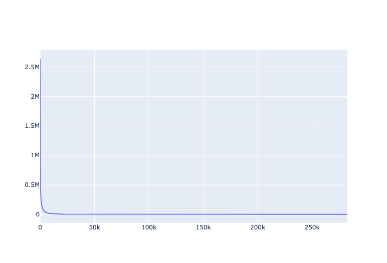
In fact, this looks very much like the probability density function of the Pareto distribution (see Wikipedia article). However we can already see from that graph, that there are very few movies with very high numbers of votes, and then there are loads of movies with hardly any number of votes.
In order to get make make it easier to interpret the data, we can calculate the cumulative distribution by cumulatively adding up the number of votes, which we can do with the .cumsum() function from Pandas.
movie_data['cumsum'] = movie_data['numVotes'].cumsum()
movie_data
| tconst | titleType | primaryTitle | originalTitle | isAdult | startYear | endYear | runtimeMinutes | genres | averageRating | numVotes | row_num | cumsum | |
|---|---|---|---|---|---|---|---|---|---|---|---|---|---|
| 82427 | tt0111161 | movie | The Shawshank Redemption | The Shawshank Redemption | 0.0 | 1994.0 | NaN | 142 | Drama | 9.3 | 2639333 | 0 | 2639333 |
| 251144 | tt0468569 | movie | The Dark Knight | The Dark Knight | 0.0 | 2008.0 | NaN | 152 | Action,Crime,Drama | 9.0 | 2610926 | 1 | 5250259 |
| 634176 | tt1375666 | movie | Inception | Inception | 0.0 | 2010.0 | NaN | 148 | Action,Adventure,Sci-Fi | 8.8 | 2314403 | 2 | 7564662 |
| 99042 | tt0137523 | movie | Fight Club | Fight Club | 0.0 | 1999.0 | NaN | 139 | Drama | 8.8 | 2083152 | 3 | 9647814 |
| 81333 | tt0109830 | movie | Forrest Gump | Forrest Gump | 0.0 | 1994.0 | NaN | 142 | Drama,Romance | 8.8 | 2043215 | 4 | 11691029 |
| ... | ... | ... | ... | ... | ... | ... | ... | ... | ... | ... | ... | ... | ... |
| 1126913 | tt6555682 | movie | Janata Express | Janata Express | 0.0 | 1981.0 | NaN | NaN | Drama | 6.4 | 5 | 282326 | 996061058 |
| 552959 | tt11991560 | movie | Parimala Lodge | Parimala Lodge | 0.0 | 2020.0 | NaN | NaN | Drama | 8.8 | 5 | 282327 | 996061063 |
| 552848 | tt11989824 | movie | Jeeva (2009 film) | Jeeva (2009 film) | 0.0 | 2009.0 | NaN | NaN | Romance | 5.4 | 5 | 282328 | 996061068 |
| 552567 | tt11984548 | movie | The Old House | O Casarão | 0.0 | 2021.0 | NaN | 72 | Documentary | 8.4 | 5 | 282329 | 996061073 |
| 1180256 | tt7738732 | movie | La settima onda | La settima onda | 0.0 | 2015.0 | NaN | NaN | Drama | 6.4 | 5 | 282330 | 996061078 |
282331 rows × 13 columns
Let's plot this.
fig = go.Figure(data=[go.Scatter(x=movie_data['row_num'], y=movie_data['cumsum'])])
fig.show()

That looks good. We can now use that data to calculate which percentage of the total votes the first 20% of movies receive.
First, we get the total number of movies and votes.
rows, cols = movie_data.shape
print(rows, cols)
282331 13total_movies = rows
total_votes = movie_data.iloc[rows-1, cols-1] # 'cumsum' of last row
print(total_movies, total_votes)
253451 835070653Let's get the movie number that marks the first 20%. We use the python function math.floor() to get an integer value.
from math import floor

num_movies_20perc = floor(total_movies * .2)
num_movies_20perc
56466From the this row of the movie dataframe, we can now extract the cumulative number of votes of the first 20% of movies.
cum_votes_20perc = movie_data.iloc[num_movies_20perc, cols-1]
cum_votes_20perc
977776286Now we can calculate the percentage of votes that the first 20% of movies recieve.
perc = cum_votes_20perc / total_votes
perc
0.9816429008181765That means that 98.2% of all votes on IMDb go to only 20% of the movies! The remaining 80% of movies receive only 1.8% of all votes!
With that remarkable insight (feel free to use it as a fun fact of the day and tell your colleagues) this tutorial has reached it's
-- END --
Thanks for following along, I hope you found it interesting. If you have any questions or feedback, please leave a comment below!
As a bonus, here are a couple of ideas for further explorations:
- scatterplot of averageRating vs numVotes (be careful not to try plotting the unfiltered dataset, this might crash your browser, believe me, I've tried)
- bar chart of number of movies per year
- average runtime per year or category
- explore the other IMDb datasets, like
title.principalsortitle.crew, to investigate popular actors, directors etc.